Big-O Notation Explained: Complexity Analysis
Aug 20, 2024
Table of Contents
Introduction
Algorithm analysis is an important topic in computer science. It is also frequently asked in the interviews. In my Meta interview, I was asked to analyze and explain the time and space complexities of all of the code pieces that I wrote.
To design efficient algorithms as computer engineers, we need to be able to analyze their complexity. We use the Big-O notation to analyze algorithms’ growth in terms of space and time.

We can informally define the algorithm as a black box between input and output. An algorithm defines a step-by-step procedure to solve a computational problem. In most cases, the algorithm is not specific to an input, it is general and can be applied to a range of inputs. Each distinct input is an instance of the problem.
As a software architect, we should know that our resources are scarce. We do not have infinite memory, or infinite time to run our algorithms.
- Algorithm
- A step-by-step procedure to solve a computational problem.
- Instance
- A distinct input to an algorithm.
- Resource
- Memory, time, and other scarce resources that are used by an algorithm.
Consider a case where we need to develop an algorithm. The algorithm should output a result in 5 seconds and should use less than 1 GB of memory. Let’s say that an inefficient algorithm uses 0.1 seconds and 0.1 GB of memory. Even though this inefficient algorithm meets the requirements, we would still want to develop a more efficient algorithm because:
- Scalability: The input size may increase in the future and the inefficient algorithm may not meet the requirements. As we will see, the inefficient algorithm may not scale well.
- Cost: The inefficient algorithm would be more costly to run.
- Energy: The inefficient algorithm would consume more energy.
Big-O Notation
Big-O notation is a symbol used to describe the asymptotic behavior of a function. In the context of algorithm analysis, Big-O notation is used to describe the growth of an algorithm in terms of space and time. Without going into details we can say that Big-O notation is used to describe the worst-case behavior of an algorithm.
Let’s see some examples:
- O(1): Constant time or space. The algorithm always runs in a constant time or uses a constant space. However, this does not mean that the algorithm runs in 1 unit of time. The algorithm might take billion years to run but if its runtime does not depend on the input size, we say that it runs in constant time.
- O(n): Linear time or space. If the input is doubled, the runtime or the space is also doubled.
- O(n^2): Quadratic time or space. If the input is doubled, the runtime or the space is quadrupled.
- O(log n)
- O(n log n)
- O(2^n)
- O(n!)
- I think you get the idea.
Since we deal with the asymptotic behavior of the algorithm, we do not care about the constants or the lower terms:
- O(2n) = O(n)
- O(3n^2 + 2n + 1) = O(n^2)
- O(5 log n) = O(log n)
- O(10n log n) = O(n log n)
- O(1000) = O(1)
- O(1000n + n^(1/2)) = O(n)
Sorting a list with a trillion elements has the same Big-O notation as sorting a list with 10 elements. This is because the Big-O notation describes the growth of the algorithm, not the actual runtime. So, we do not care about particular instances of the problem.
Complexity Analysis Intuition

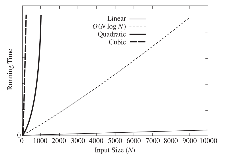
The chart above is very powerful for understanding the Big-O notation. Even though the line for O(nlogn) looks linear it is not. The chart perfectly illustrates how the growth of the algorithms makes huge differences for large input sizes.
Let’s say, we have a task that takes 1 second for 10 elements and we increase the input size to 1000. If the algorithm we designed for this task is:
- O(n): It will take 100 seconds.
- O(n^2): It will take approximately 2 hours and 45 minutes.
- O(2^n): It will take more than the age of our universe multiplied by one trillion years.
It is a long time, right? This is why we need to design efficient algorithms.
Code Examples
Let’s see some code pieces and analyze their complexity.
Constant Time: O(1)
- Print Hey: The following code prints “Hey”. The time complexity of this code is O(1) because it always runs in constant time.
def print_hey():
print("Hey")- Print Hey 1000000 times: The following code prints “Hey” 1000000 times. The time complexity of this code is O(1) because it always runs in constant time.
def print_hey():
    for i in range(1000000):
print("Hey")Linear Time: O(n)
- Sum of n numbers: The following code calculates the sum of the first n numbers. The time complexity of this code is O(n) because the loop runs n times. You might say that “There is a constant time where we set the total to 0.”. However, remember that we are interested in the growth of the algorithm. O(n + 1) = O(n).
def sum_of_n(n):
    total = 0 # O(1)
    for i in range(1, n + 1):
        total += i
return total- Linear Search: The following code searches for an element in a list. We could find the element in the first iteration or in the last iteration. However, we are interested in the worst-case scenario. Hence, the time complexity of this function is O(n).
def linear_search(arr, x):
    for i in range(len(arr)):
        if arr[i] == x:
            return i
return -1- Sum of Twice: Careful! This is O(n) as well.
def sum_of_twice(arr):
    total = 0
    for i in range(len(arr)):
        total += arr[i]
    for i in range(len(arr)):
        total += arr[i]
return total- Double Loop: Don’t try to find the complexity by counting the number of nested loops. This is O(n) as well.
def double_loop(arr):
    for i in range(len(arr)):
        for j in range(1000):
            print(arr[i])
    return
Quadratic Time: O(n^2)
- Sum of all pairs: The following code calculates the sum of all pairs in a list. The time complexity of this code is O(n^2).
def sum_of_all_pairs(arr):
    total = 0
    for i in range(len(arr)):
        for j in range(len(arr)):
            total += arr[i] + arr[j]
return total- Sum of all distinct pairs: The following code calculates the sum of all distinct pairs in a list.
If you are careful, you can say that the time complexity of this code is not O(n^2) since for an arr with size 2, the loop runs 1 time and for an arr with size 4, the loop runs 6 times. You might calculate the time complexity as O((n)*(n+1)/2), but in Computer Science, what we are interested in is the growth of the algorithm and it is proportional to n^2. Hence, the time complexity of this code is O(n^2).
def sum_of_all_distinct_pairs(arr):
    total = 0
    for i in range(len(arr)):
        for j in range(i + 1, len(arr)):
            total += arr[i] + arr[j]
    return total
Logarithmic Time: O(log n)
- Binary Search: The following code searches for an element in a sorted list. Binary search works by splitting the search space in half in each iteration. This is a common theme for the algorithms that have logarithmic time complexity.
def binary_search(arr, x):
    low = 0
    high = len(arr) - 1
    while low <= high:
        mid = (low + high) // 2
        if arr[mid] == x:
            return mid
        elif arr[mid] < x:
            low = mid + 1
        else:
            high = mid - 1
return -1- Logarithmic Loop: The following code prints the elements of an array in a logarithmic way.
def logarithmic_loop(arr):
    i = 1
    while i < len(arr):
        print(arr[i])
        i *= 2
Linearithmic Time: O(n logn)
- Quick Sort: The following code sorts an array using the quick sort algorithm. It is a divide-and-conquer algorithm that has an average time complexity of O(n logn). You can think of it as “logn operations for each n element”. Hence, the time complexity is O(n logn).
def quick_sort(arr):
    if len(arr) <= 1:
        return arr
    pivot = arr[len(arr) // 2]
    left = [x for x in arr if x < pivot]
    middle = [x for x in arr if x == pivot]
    right = [x for x in arr if x > pivot]
    return quick_sort(left) + middle + quick_sort(right)
Merge Sort and Heap Sort are other examples of algorithms that have O(n logn) time complexity.
Exponential Time: O(2^n)
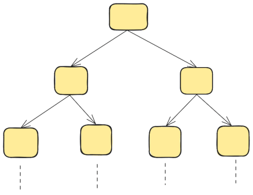
- Fibonacci: You can visualize this algorithm as a binary tree where at each level the number of nodes doubles. Hence, the complexity of this code is O(2^n).
def fibonacci(n):
    if n <= 1:
        return n
    return fibonacci(n - 1) + fibonacci(n - 2)
Factorial Time: O(n!)
- Permutations: You have n! permutations of a list. The time complexity is O(n!).
def permutations(arr):
    if len(arr) == 0:
        return [[]]
    result = []
    for i in range(len(arr)):
        rest = arr[:i] + arr[i + 1:]
        for p in permutations(rest):
            result.append([arr[i]] + p)
return resultNP-Hard and NP-Complete Problems
I won’t explain these concepts in detail but I want to mention them for the sake of completeness. We can characterize NP-Complete problems with three properties:
- No efficient algorithm is known for solving them.
- No one has been able to prove that an efficient algorithm does not exist.
- If we can solve one of them efficiently, we can solve all of them efficiently.
Quite interesting, right? If you are interested in this topic, you can read more about it from the references.
Famous Examples of NP-Complete problems are:
- Traveling Salesman Problem
- Knapsack Problem
- Graph Coloring Problem
- Hamiltonian Cycle Problem
Conclusion
Complexity analysis is an essential topic in computer science. We talked about its importance and the fact that we have scarce resources. Then, we introduced the Big-O notation with common complexities. We also saw some code examples and analyzed their time complexities.
If you have any questions or feedback, feel free to reach out to me from the links on the sidebar.
References
- Cormen, T. H., Leiserson, C. E., Rivest, R. L., & Stein, C. (2009). Introduction to Algorithms, third edition. http://portal.acm.org/citation.cfm?id=1614191
- Weiss, M. A. (2012). Data structures and algorithm analysis. https://ci.nii.ac.jp/ncid/BA28306929
